Method 9.1 adaptive margin

M9.1 uses only branch 2 and branch 3: a complex closed-loop FRF where the command excites the loop, plus residual output growth for output-only evidence. All plotted and reported times are causal window-end times. Branch 1 is ignored.

Input-excited band

Use branch 2 when \(dd_{\mathrm{lead}}\) has enough power and coherence is acceptable. The estimator reads the command-correlated transfer and converts the complex \(S,T\) pair into an NCF distance.

\[ \widehat T(\omega,t)=\frac{\Phi_{yu}(\omega,t)}{\Phi_{uu}(\omega,t)},\qquad \widehat S(\omega,t)=1-\widehat T(\omega,t) \]

Residual branch

Use branch 3 for output-only evidence. The normal path searches input-quiet bins; a frequency-matched early-warning path may scan the full band when the direct S,T branch is already moving at the same frequency.

\[ \Phi_{\mathrm{res}}(\omega,t)\approx \Phi_{yy}(\omega,t)\left(1-\gamma^2(\omega,t)\right) \]

Notation

Let \(u=dd_{\mathrm{lead}}\), \(y=dm\), \(d\) be internal disturbance or noise, \(H\) be the plant path from command force/displacement action to measured displacement, and \(C\) be the controller.

\[ L(\omega,t)=C(\omega)H(\omega,t),\qquad S(\omega,t)=\frac{1}{1+L(\omega,t)},\qquad T(\omega,t)=\frac{L(\omega,t)}{1+L(\omega,t)} \]

The measured output is the sum of a command-correlated part and an internally excited part:

\[ y(\omega,t)=T(\omega,t)u(\omega,t)+S(\omega,t)d(\omega,t) \]

Here \(\Phi_{ab}\) means the cross-spectrum between signals \(a\) and \(b\), and \(\Phi_{aa}\) is the autospectrum of \(a\).

Branch 2: input-excited band

Step 1: require identifiable input power

M9.1 only trusts branch 2 on bins where the input has enough power and the estimated input-output relation is coherent:

\[ \Omega_{\mathrm{exc}}(t)= \left\{\omega: \Phi_{uu}(\omega,t)\ \text{is large enough},\quad \gamma^2(\omega,t)\ge \gamma_{\min} \right\} \]

Step 2: estimate the command-correlated transfer

Using the output equation, the cross-spectrum with the command is:

\[ \Phi_{yu}(\omega,t)= T(\omega,t)\Phi_{uu}(\omega,t) +S(\omega,t)\Phi_{du}(\omega,t) \]

If the internal disturbance is not correlated with the command, \(\Phi_{du}\approx0\). Then:

\[ \widehat T(\omega,t)= \frac{\Phi_{yu}(\omega,t)}{\Phi_{uu}(\omega,t)} \approx T(\omega,t) \]

Step 3: convert \(S,T\) into margin

For unity feedback, \(S=1-T\). The NCF loop distance at one frequency can be written directly from \(S,T\):

\[ b(\omega,t)= \frac{1}{\sqrt{2}\sqrt{|S(\omega,t)|^2+|T(\omega,t)|^2}} \]

M9.1 uses the largest distance over qualified excited/coherent bins:

\[ \tilde b_{ST}(t)= \frac{1}{\sqrt{2}\, \max_{\omega\in\Omega_{\mathrm{exc}}(t)} \left(\sqrt{|\widehat S(\omega,t)|^2+|\widehat T(\omega,t)|^2}\right)} \]

A small finite-window correction sharpens sub-nominal branch-2 margins while leaving the healthy nominal point anchored:

\[ b_{ST}(t)= b_0\left(\frac{\tilde b_{ST}(t)}{b_0}\right)^{1.15},\qquad \tilde b_{ST}(t)

This branch is the phase-aware branch. If the dangerous frequency is externally excited, it can detect margin loss caused by phase delay even before a large output-only resonance is visible.

Branch 3: residual output evidence

Step 1: decompose the output spectrum

When \(u\) and \(d\) are approximately uncorrelated, the total output spectrum is:

\[ \Phi_{yy}(\omega,t)= \underbrace{|T(\omega,t)|^2\Phi_{uu}(\omega,t)}_{\text{command-correlated output}} + \underbrace{|S(\omega,t)|^2\Phi_{dd}(\omega)}_{\text{residual/internal output}} \]

Step 2: use coherence to remove the command-correlated part

\[ \gamma^2(\omega,t)= \frac{|\Phi_{yu}(\omega,t)|^2} {\Phi_{uu}(\omega,t)\Phi_{yy}(\omega,t)} \]

The residual output spectrum is approximated as:

\[ \Phi_{\mathrm{res}}(\omega,t)\approx \Phi_{yy}(\omega,t)\left(1-\gamma^2(\omega,t)\right) \]

Step 3: search residual growth

Branch 3 compares the current residual spectrum with the healthy reference spectrum. The normal fallback searches outside the branch-2 excited/coherent bins:

\[ \Omega_{\mathrm{quiet}}(t)=\Omega_{\mathrm{wide}}\setminus\Omega_{\mathrm{exc}}(t),\qquad q(t)= \max_{\omega\in\Omega_{\mathrm{quiet}}(t)} \frac{\Phi_{\mathrm{res}}(\omega,t)} {\Phi_{\mathrm{res,ref}}(\omega)} \]

Then it maps the residual growth to a conservative margin proxy:

\[ b_{\mathrm{wide}}(t)= b_0\sqrt{\frac{q_{\mathrm{ref}}}{q(t)}} \]

For faster damage-reduction detection, M9.1 also checks a full-band residual candidate. It is accepted only when it binds within 4.0 Hz of the direct S,T branch and S,T has already moved below nominal but not below the relative alarm level. In that case the residual candidate is bounded below by 80% of the direct S,T margin.

Why this sees what branch 2 can miss

If a mode grows from internal disturbance or noise, then the residual spectrum contains:

\[ \Phi_{\mathrm{res}}(\omega,t)\approx |S(\omega,t)|^2\Phi_{dd}(\omega) \]

So branch 3 can catch output-only resonance growth when the command has almost no power at that frequency, and the bounded early-warning path can also catch the first residual growth at an already-observed S,T frequency:

\[ \Phi_{uu}(\omega)\approx0 \]

Final branch selection

M9.1 computes no known-mode peak/floor branch. Each window keeps only the lower margin from branch 2 and branch 3:

\[ b_{M9.1}(t)=\min\left(b_{ST}(t), b_{\mathrm{wide}}(t)\right) \]

This makes branch 3 the only output-only fallback. There is no branch-1 peak mask, no branch-1 calibrated proxy, and no final minimum against a branch-1 estimate.

True NCF references

Healthy true NCF0.588

Damaged true NCF0.344

Damage time10.0 s

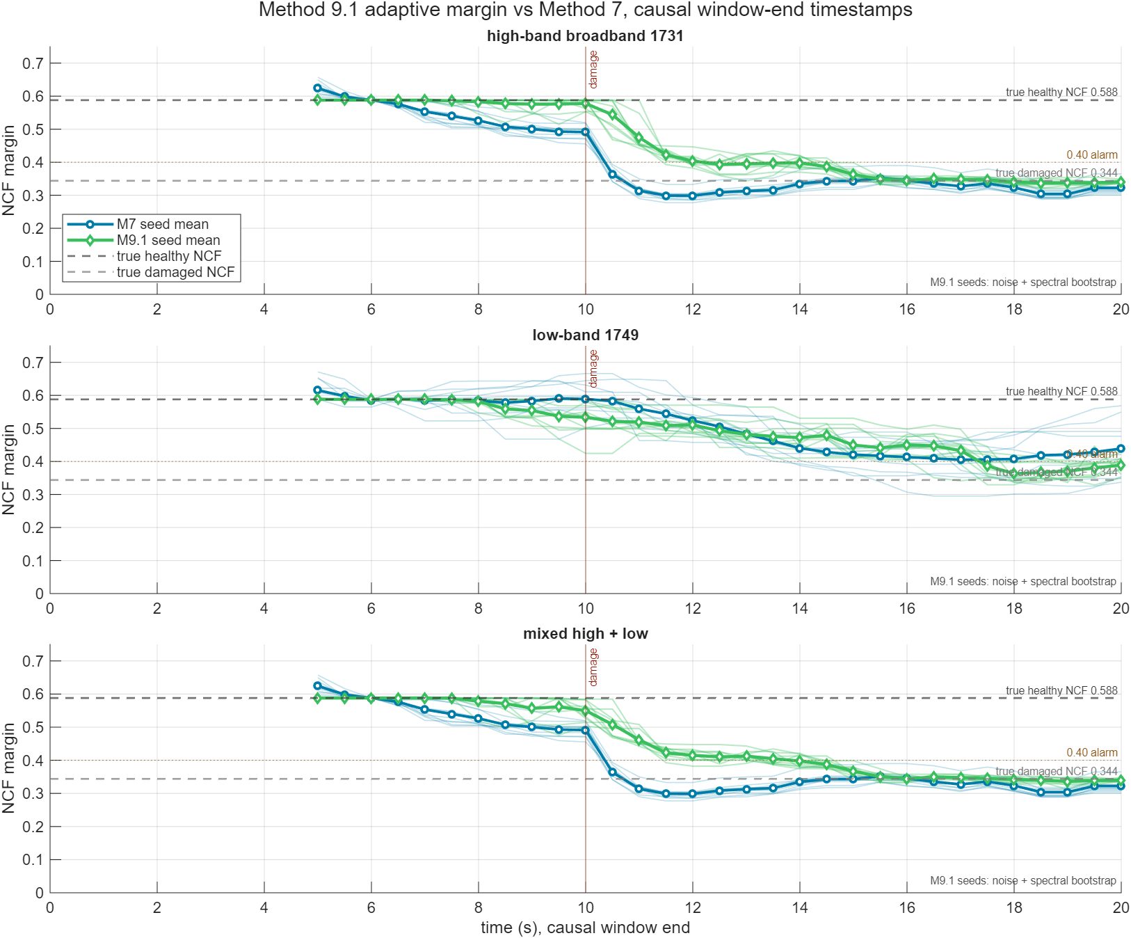
The dashed horizontal lines in the seed plot are these true loop-only NCF values, not seed-dependent estimates.

Seed spread

M9.1 seed spread includes injected noise/disturbance variability plus a bootstrap perturbation of the spectral subsegments. It is still not a full model-uncertainty interval, but it avoids plotting a deterministic averaged estimator as if finite-window spectral uncertainty were zero.

Between seeds, the plant, controller, damage timing, and command profile are fixed. What changes is the disturbance/noise realization, and for M9.1 the spectral-bootstrap perturbation used inside each finite-window estimate. The differences below are therefore estimator/data-window variability around the same true NCF values.

Case	What differs	M9.1 damaged seed range	M9.1 max seed spread	M9.1 detection range	M7 damaged seed range	M7 detection range
high-band	noise realization + M9.1 spectral bootstrap	0.340-0.353	0.146	10.5-11.5 s	0.310-0.370	11.0-12.0 s
low-band	noise realization + M9.1 spectral bootstrap	0.380-0.434	0.164	9.5-17.5 s	0.316-0.495	12.5-18.0 s
mixed	noise realization + M9.1 spectral bootstrap	0.340-0.353	0.117	10.5-11.5 s	0.310-0.370	11.0-12.0 s

Damaged seed range is the per-seed mean after the estimator buffer has cleared the damage step. Max seed spread is the largest vertical separation between M9.1 seed traces at any plotted timestamp.

Table comparison

Case	M7 damaged	M7 err	M7 seeds	M9.1 damaged	M9.1 err	M9.1 seeds	M9.1 freq	M7 ms	M9.1 ms	M9.1/M7
high-band	0.329	0.015	10/10	0.345	0.001	10/10	38.0 Hz	95	66	0.70x
low-band	0.417	0.073	10/10	0.407	0.063	10/10	37.0 Hz	76	50	0.66x
mixed	0.329	0.015	10/10	0.346	0.002	10/10	38.0 Hz	69	47	0.68x

Seed plots

Interpretation

M9.1 improves the three-case comparison by matching M7's damage-reduction timing while preserving the direct phase-aware branch. The residual branch is normally input-quiet, with a frequency-matched early-warning path bounded by the direct S,T estimate; branch 1 is no longer computed or selected.